Signal Analysis Screen Layout and Checking Waveforms
Screen Layout
In Signal Analysis, select the analysis source at the top and examine information for the same time using the central graphs, Values on the right, and results below. Graph and result regions are not shown until a log is selected.
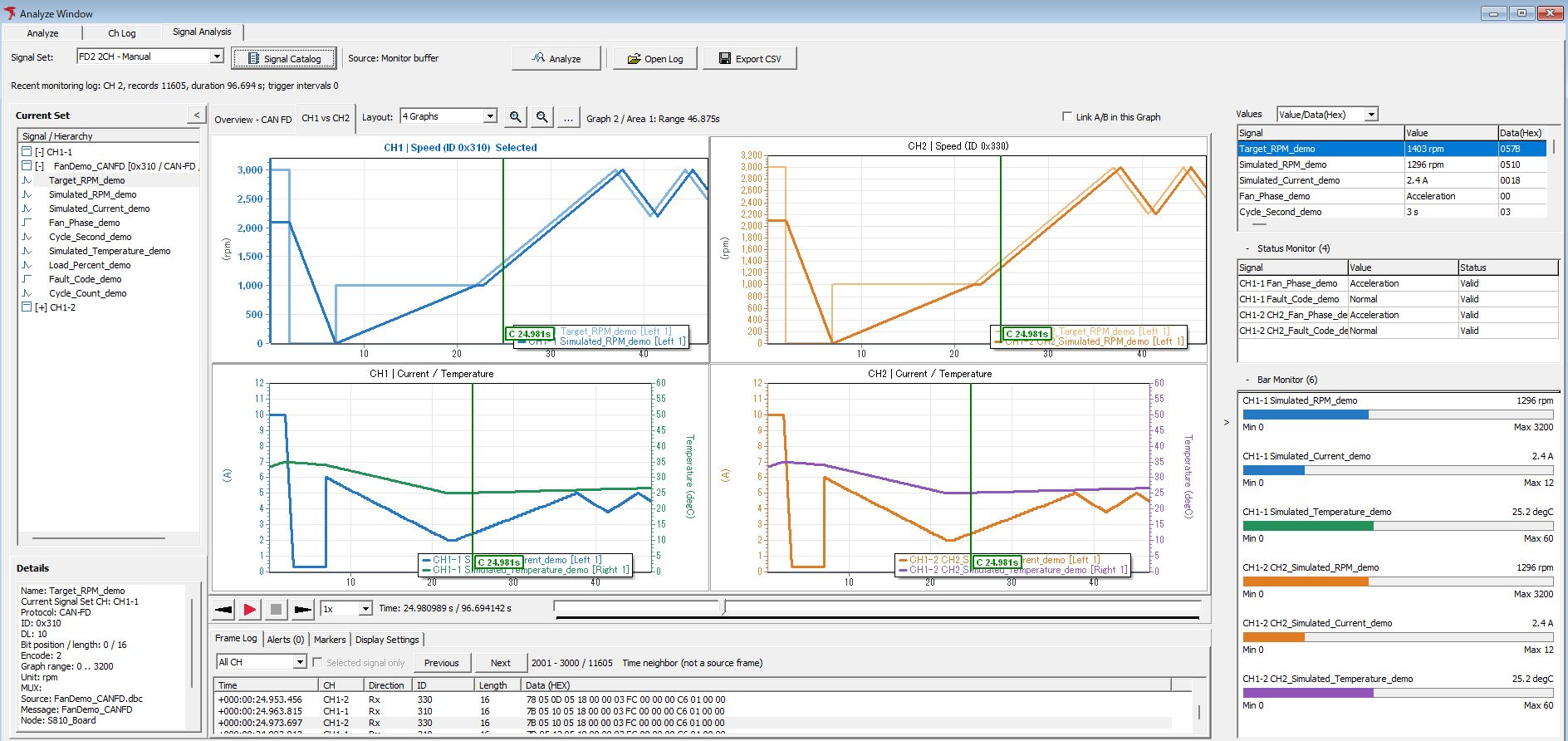
The example uses FanDemo_CANFD.dbc to compare ID 0x310 on CH1 with ID 0x330 on CH2. Current Set and Details are on the left, four graphs in the center, Values/Status Monitor/Bar Monitor on the right, and tabs such as Frame Log at the bottom. Alerts is 0. Graph tab names depend on settings; here they are “Overview - CAN FD” and “CH1 vs CH2.”
| Region / item | Operations and checks |
|---|---|
| Signal Set / Signal Catalog | Use “Signal Set” to select the Set for the next analysis. Use “Signal Catalog” to check or edit analysis definitions and channel assignments. |
| Source / Analyze | Analysis source and controls for initial analysis/reanalysis. Check that the adjacent Source identifies the intended log. |
| Open Log / Export CSV | Load communication logs and export analyzed signal values to CSV. |
| Current Set / Details | Select a signal in the hierarchy and check its definition or information about the selected item. |
| Graph 1 / Graph 2 | Switch waveform destinations. Use Layout to choose one view, two vertically/horizontally split views, or four views. |
| Values | Check signal values at the cursor time. Switch between Time/Value and Value/Data(Hex) to compare values and data. |
| Display Settings | Adjust display destinations, graph assignments, and other settings. Display concepts are shared with Signal Window. |
| Frame Log | Shows frames used for analysis. Selected signal only filters to frames related to the selected signal. |
| Alerts (count) | Check alert detections. Use “Show on graph” to toggle graph overlays. |
| Markers | Check A/B marker times, differences, and annotations. |
| Playback controls | Examine recorded log values by moving in time, changing playback speed, and pausing. No data is transmitted onto the bus. |
Selecting another Signal Set after analysis completes changes the next analysis target while the graph and Values retain the previous results. Export CSV is disabled until reanalysis finishes. See the Fan Demo - CAN FD to RPM Set example for the four-area results retained while pending and the two-signal RPM graph after Analyze.
Zooming In on Waveforms
- Select the target signal, Graph tab, and Area.
- Check displayed signals, axes, time range, and other settings in Graph Settings. For shared configuration methods, see Graph Display Settings.
- Change the displayed time-axis range using Zoom In/Zoom Out. Restore the range with Zoom Reset under More Graph commands.
- Move the cursor to the time of interest and check Values and Frame Log. If you cannot find the target in Frame Log, also check the selected-signal filter.
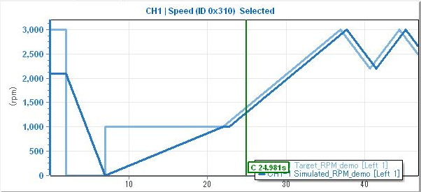
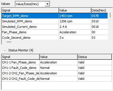
The images show a cursor at about 24.981 seconds and values at that time. Values uses Value/Data(Hex) to display physical values alongside data.

A row labeled “Time neighbor (not a source frame)” is near the cursor time. It does not identify the source frame that generated the selected signal's value. Check the channel, ID, time, and selected-signal filter when comparing.
Changing the waveform display range does not delete source log data or reduce the number of analysis input frames.
Arrange Signals Automatically
In Signal Analysis, select the destination Graph tab and open “Graph Settings” → “Auto arrange...”. Check the unassigned signals you want to plot and review “Proposed layout.” Select “Use layout” and click “OK” to apply it. See Arranging Unassigned Signals Automatically for details on eligible signals and the layout proposal.
If you switch Sets after completing an analysis, “Graph Settings” edits the Set for the next run. Check the Set name in the dialog, then click “Analyze” and wait for it to finish before checking that Set’s waveforms. The graph shows the previous results while reanalysis is pending.
Check Axes in a Range Without Samples
After analysis completes, the axes configured for signals in the selected graph remain visible when the time range has no samples to plot. The axis units, scale, and state labels reflect display settings. To check signal values, verify the Graph, Area, and time range, then move to a time with samples and compare Values with Frame Log.
Comparing with A/B Markers
- Right-click the starting position on the graph and select “Set A here.”
- Select “Set B here” at the ending position.
- Check A/B times, time difference, and target signal values in Markers.
- To remove one marker, use “Clear A” or “Clear B.” To remove both, select “Clear A/B in this Area” when linking is disabled, or “Clear linked A/B in this Graph” when enabled.
Check the target Graph and Area before operating markers. Enabling “Link A/B in this Graph” links A/B markers within the same Graph for comparison. Do not confuse them with markers in another Graph.
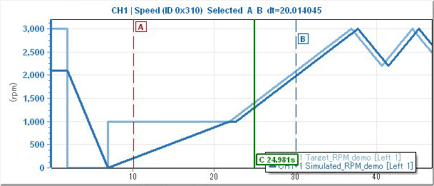
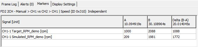
The example compares two times in the same Area for CH1. The time difference is 20.014045 seconds. Target_RPM_demo changes from 1000 rpm to 2088 rpm, a difference of 1088 rpm.
Checking Alert Occurrences
Check alert conditions in the analysis Set, then select a detection time and target in “Alerts” to compare waveforms and values. For condition types, thresholds, durations, and recovery conditions, see Alert Settings. If conditions change, check the state after reevaluation/reanalysis.
- Stop monitoring, select a row in Alert History, and click “Open in Signal Analysis.” Alternatively, specify the target log and conditions in Signal Analysis and run analysis.
- Open “Alerts” below and check Signal, rule name, activation/recovery times, and values in the detection row. Figure 1 shows results analyzed with the same condition configured in Set “FD2 2CH - Manual.”

Figure 1. Alert detection row in Signal Analysis.
Alerts contains 1 item, State is Recovered, and Rule is CH1 RPM High. Activation is at +000:00:01.264.351 with 2200 rpm, recovery is at +000:00:31.480.286 with 2092 rpm, and the calculated duration is 30.215935 s. Rule Type is Monitoring.
- Double-click the detection row to move the cursor to the activation time. Compare the signal's waveform and Values. Use “Show on graph” to toggle the alert overlay.
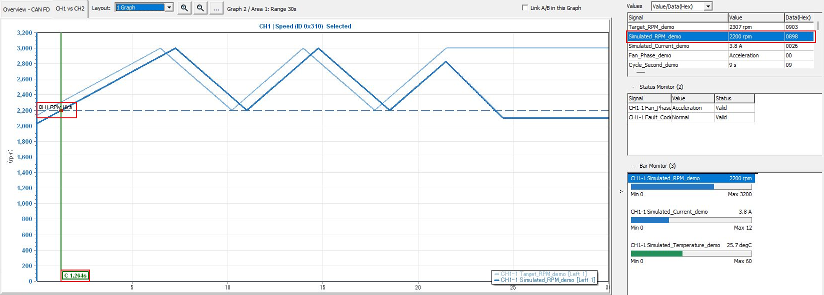
Figure 2. Waveform and Values at the alert time.
Figure 2 examines actual rotational speed on CH1-1, ID 0x310. The red point on the waveform is CH1 RPM High, and the green C marker is at about 1.264 s. Values shows Simulated_RPM_demo at 2200 rpm, Data(Hex) 0898, matching Start Value in the detection row.
“Alerts” shows results for the selected analysis log and conditions. Distinguish these from Alert History accumulated during monitoring and from Signal Trigger, which starts/stops log recording.
Adding Annotations
Right-click the graph, select “Add Annotation Here,” and configure Time (seconds), Title, and optionally Comment in Annotation. Double-click an annotation row in Markers to jump to its time. Right-click the row and use Edit Annotation to modify it.
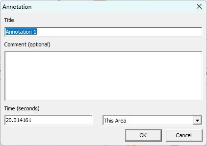

The example adds “Annotation 1” at 20.014161 seconds. Also check the display scope. This Area shows the annotation in the target Graph/Area.
Annotations are retained within the session for the currently open log. Record any required times, titles, and comments separately before switching logs. Do not assume annotations are saved in MPXSIG or analysis CSV files.