Graph Display Settings
Overview
Graphs are divided into two tabs, each containing up to four Areas. Configure destinations per signal and compare multiple signals using shared axes in the same Area. Newly configured Sets support up to 32 graph signals across the entire Set. Assignments in Areas not currently visible also count; assigning the same signal to multiple Areas still counts as one signal.
Assigning Signals to Graphs
- Stop monitoring and open Edit for the target signal in Signal Catalog.
- Turn on Graph under Conversion / Display and click the “Graph” button.
- At the top of the Graph dialog, select Graph 1/Graph 2 and the target Area.
- Signals and axes lists the signal being edited in Signal Setting. Select its checkbox.
- Check the signal/axis counts for the selected Area and assignments in the list.
- Adjust shared-axis settings under Selected axis if needed.
- Confirm the Graph dialog with OK, then confirm the parent Signal Setting with OK too.
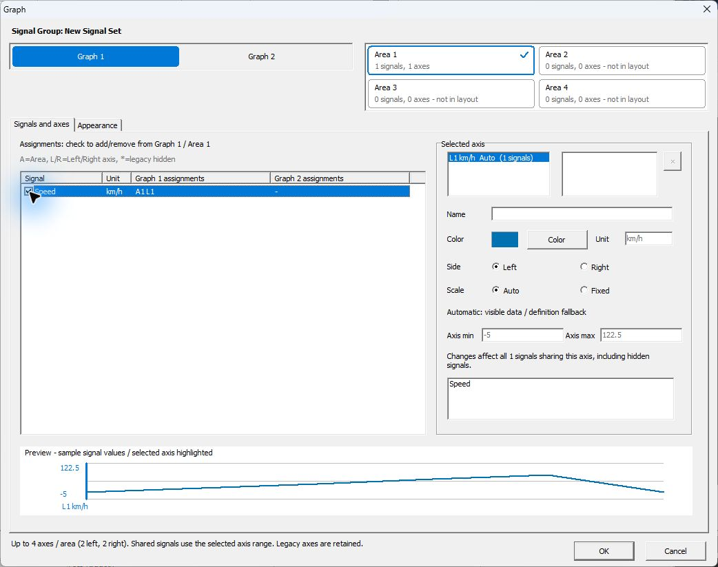
Figure 1. Example assignment of Speed to the left axis of Graph 1, Area 1.
Figure 1 assigns Speed in New Signal Set to Area 1 of Graph 1. Area 1 shows 1 signals and 1 axes, and Speed's Graph 1 assignments shows A1 L1. L1 under Selected axis is the first left-hand axis, with unit km/h. Preview at the bottom uses sample values to check settings, not waveforms acquired from actual communication.
To display the same signal in another Area, switch destinations at the top and select its checkbox there as well. Checkbox operations apply to the currently selected Graph and Area.
To assign multiple signals in a Set together, open graph settings using “Graph Settings...” in Signal Window.
A shared axis lets multiple signals in the same Area use the same scale. Initially, assign one signal to one Area, then share axes when needed.
Auto Arranging Unassigned Signals
Use automatic layout to add signals to a graph. It keeps existing assignments and can propose a layout for an empty graph.
- Stop monitoring. If the target Set is not current, open Signal Catalog, select the Set, click
Set Current, and close the Catalog. In Signal Window, verify the Set shown in theSignal Setfield and select the graph tab (Graph 1orGraph 2). - Open
Graph Settings.... Check the target graph tab and clickAuto arrange.... - Under
Signals to add, select the signals you want to display. Check the target Set and Graph at the top and review the Areas, axes, and series inProposed layout. A selected signal with monitoring turned off is markedEnable Monitor. - Click
Use layoutto bring the proposal into Graph Settings. Check the assignments there, then clickOKto apply them. Applying the layout turns on monitoring for signals markedEnable Monitor.
Figures 2 and 3 use New Signal Set with Speed added and assigned to CH1-1. Speed belongs to SensorFrame with LIN ID 10 (0x10) and uses km/h. Starting with no graph assignments, select Graph 1 and auto arrange Speed only. If the channel is unassigned, first configure Set membership and channel assignment.
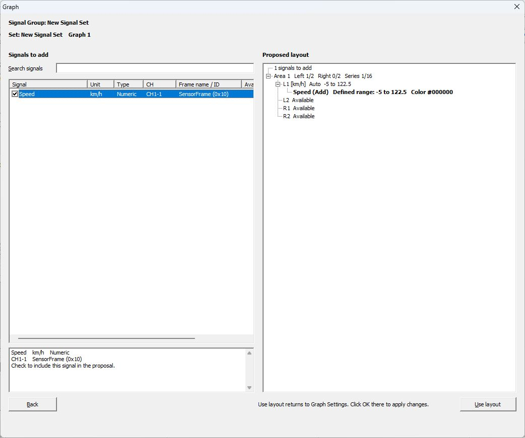
Figure 2. Select Speed and check the proposal for Area 1, L1 under Proposed layout.
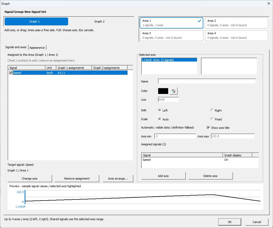
Figure 3. Graph Settings after Use layout, before clicking OK.
In Figure 3, Speed's Graph 1 assignments shows A1 L1, and Selected axis shows L1 km/h Auto (1 signals). Click OK to apply the settings. Preview at the bottom uses sample values to check settings, not waveforms acquired from actual communication.
Signals without a channel assignment, signals with an unassigned channel dependency, and signals already assigned to a graph (including hidden assignments) cannot be selected. Check Availability for the reason. If there is not enough room on the available axes or for the series, reduce the selection or review the existing layout and assignments in Graph Settings.
You can also open the same tool with signals preselected: select the rows in the Signal Window signal list, right-click, and choose Auto arrange selected signals.... Review the proposed layout and apply it in the same way.
See Changes in Ver.4.10 for other changes in this version.
Signals and axes Reference
| Item | Description |
|---|---|
| Signal Group | Shows the Set being edited. |
| Graph 1 / Graph 2 | Selects the graph tab to configure. |
| Area 1–4 | Selects the Area to configure. You can check its signal and axis counts. |
| not in layout | An Area not visible in the current layout. Check assignments together with the screen layout. |
| Signal checkbox | Configures assignment to the selected Graph/Area. |
| Graph 1/2 assignments | Shows destinations within each tab. A means Area, L/R means left/right axis, and * indicates an assigned signal with Graph turned off. |
| Selected axis | Check axes in the selected Area and signals sharing an axis. |
| Change axis / Remove assignment | Changes the selected signal's axis or removes its assignment. If it has an assignment in the current Area, that assignment is targeted. If it has only one assignment in another Area of the same tab, that assignment is targeted. If there are multiple assignments, switch to the target Area. |
| Add axis / Delete axis | Adds an unassigned numeric axis to the selected Area or deletes the selected axis. Deleting an axis also removes assignments of signals using it. |
| Name / Color / Unit | Configures the axis display name, color, and unit name. |
| Side | Places the axis on the Left or Right. |
| Scale | Selects Auto or Fixed. |
| Axis min / Axis max | Configures the display range for Fixed. |
| Preview | Shows a preview of the selected axis or signal. |
Using Shared Axes
Signals on the same axis use the same scale. Changing an axis range affects all signals sharing it. Check the signal list under Selected axis before changing settings.
To assign a numeric signal to an existing shared axis, its unit must match the axis unit exactly, including letter case. Use separate axes for signals with different units. State displays use dedicated axes. Changing a unit name does not convert physical values.
For new configurations, one Area supports up to four axes (two left, two right) and 16 signal assignments, including hidden assignments. Older settings may retain configurations exceeding the axis limit or Set-wide assigned-signal limit. Operations that increase the excess are not allowed; reduce assignments or axes to return within limits. If you cannot change assignments or axes, check the on-screen message and existing axis configuration.
Auto and Fixed
Auto adjusts the scale according to displayed data and other factors. Fixed uses the range specified by Axis min / Axis max. To compare multiple measurements on the same scale, use Fixed with the same range.
Appearance Reference
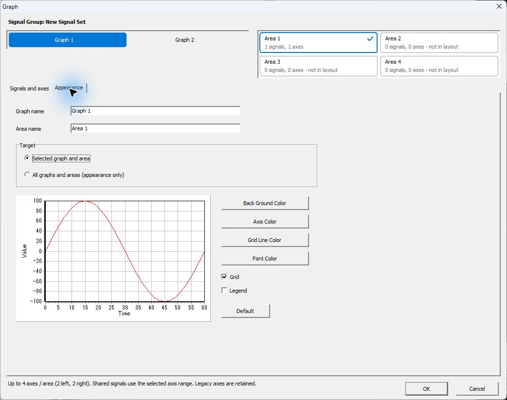
Figure 4. Example Appearance settings for Graph 1, Area 1.
| Item | Description |
|---|---|
| Graph name / Area name | Sets graph tab and Area names. |
| Selected graph and area | Edits appearance for the selected graph and Area. |
| All graphs and areas (appearance only) | Selects all graphs/Areas as the scope for appearance changes. |
| Back Ground Color | Sets the background color. |
| Axis Color / Grid Line Color / Font Color | Sets axis, grid, and text colors. |
| Grid / Legend | Configures grid/legend visibility. |
| Default | Restores default appearance settings. Check the scope before running it. |
The sample curve in Figure 4 is also an example for checking appearance.
Display Operations in Signal Window
Use Graph 1/Graph 2 and the layout selector to switch display destinations. Zooming the time range or resetting it from the “…” menu links the time axes of Areas in the same graph tab. Use Pause/Resume to pause/resume graph display.
Example: Comparing Speed's Actual Waveform and Value
Figures 5 and 6 display Speed from the sample LDF in a Set named LIN Sensor. This differs from New Signal Set in Figures 1–4, so check which Set you are configuring.
- Stop monitoring and use
Set Currentin Signal Catalog to makeLIN Sensorthe current Set. In Signal Window, open “Graph Settings...” and select Graph 1, Area 1. - Check Speed and verify that Graph 1 assignments shows
A1 L1and Selected axis showsL1 km/h Auto(Figure 5). State is not assigned to a graph in this example.
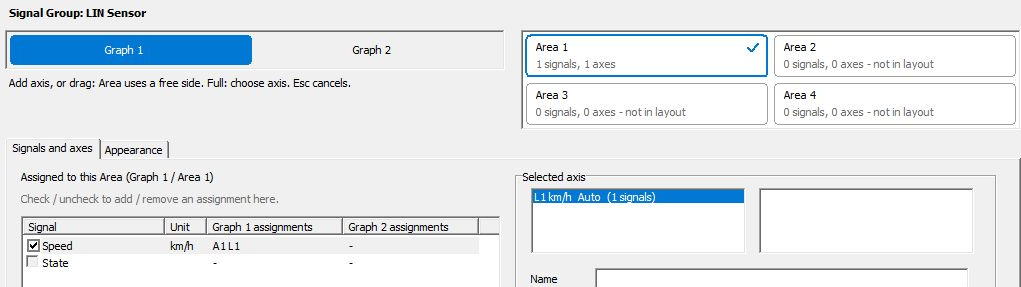
Figure 5. Assigning Speed to Graph 1, Area 1 from Graph Settings.
- Turn on Legend in Appearance and confirm the settings. Select a layout in Signal Window that shows Graph 1 and Area 1, then monitor the target communication.
- In Figure 6, check the legend
CH1-1 Speed [Left 1]and km/h on the left axis. The Auto display range is 9.5–10.5 km/h, and the black horizontal line is at 10 km/h. Values on the right also shows Speed at 10 km/h with Status Received, matching the waveform height.
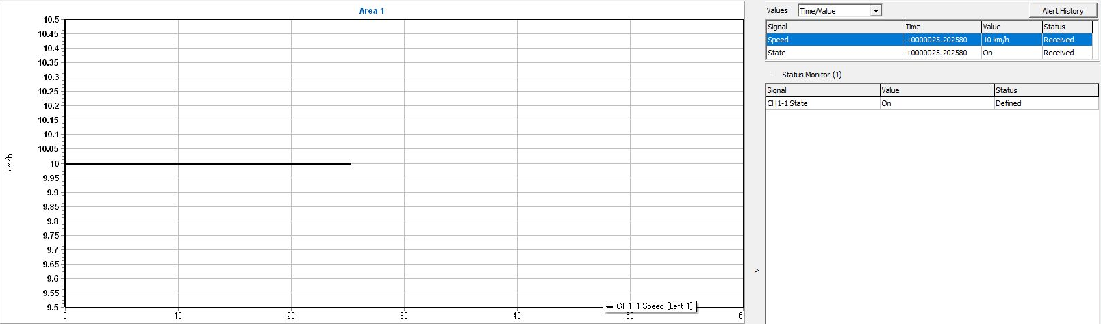
Figure 6. Comparing Speed's actual waveform and Values on the same screen.
Figure 6 shows decoded data from actual transmission of ID 0x10 with data “1E 01” as Tx every 100 ms using Master Sim. on CH1-1. Speed's Raw value 30 converts to 10 km/h. Because the transmitted data is constant, the waveform is a horizontal line at 10 km/h. Time in Values is +0000025.202580. Applying SensorSchedule from the LDF initially creates an Rx slot, so this capture changes it to Tx for transmission. For correspondence with source bytes and direction checks, see the basic operations.
Example: Comparing Two Signals with the Same Unit on a Shared Axis
Figures 7–9 show a separate capture comparing Speed and Speed_half in the Set “SensorFrame Speed.” Speed_half is a comparison derived signal calculated as Speed ÷ 2, and both signals use km/h. Speed is black and Speed_half is red.
- Stop monitoring and use
Set Currentin Signal Catalog to make “SensorFrame Speed” the current Set. In Signal Window, open “Graph Settings...”. - Assign Speed and Speed_half to the same left axis L1 in Graph 1, Area 1. If assigned to different axes, select the signal and use Change axis to select L1. Check that Area 1 shows
2 signals, 1 axesand both signals show assignmentA1 L1. - Set Scale for Graph 1 to Auto. In Figure 7, Selected axis shows
L1 km/h Auto (2 signals), and Assigned signals lists Speed and Speed_half.
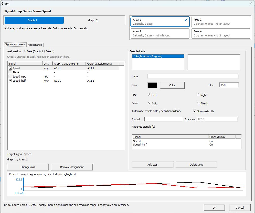
Figure 7. Example settings sharing L1 between 2 signals in the same Area.
- Assign both signals to L1 in Graph 2, Area 1 as well, set Scale to Fixed, Axis min to 0, and Axis max to 30, then confirm. The 2 signals within each Area share a scale; Scale is configured separately for Graph 1 and Graph 2.
- After configuring, capture communication and stop, then switch between Graph 1 and Graph 2. Set both displayed time ranges to 0–60 seconds.
Preview at the bottom of Figure 7 uses samples for checking settings. Figures 8 and 9 below show the same actual communication after acquisition has stopped, with only the tab switched. Both have a 0–60 second time range, allowing comparison of vertical-axis settings.
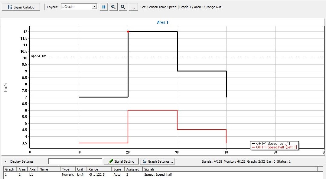
Figure 8. The same 2 signals displayed with Auto in Graph 1.
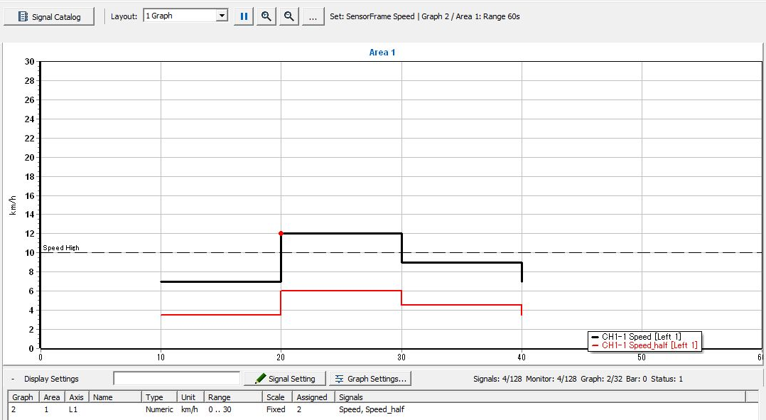
Figure 9. The same 2 signals displayed with Fixed 0–30 km/h in Graph 2.
| Time | Speed (black) | Speed_half (red) |
|---|---|---|
| 10 seconds | 7 km/h | 3.5 km/h |
| 20 seconds | 12 km/h | 6 km/h |
| 30 seconds | 9 km/h | 4.5 km/h |
| 40 seconds | 7 km/h | 3.5 km/h |
The displayed scale in Figure 8 is 3.5–12 km/h (0.5 increments), while Figure 9 uses 0–30 km/h (2 increments). Check the scale on the left of the graph for the actual Auto range. The vertical range changes the waveform's appearance, but the values at each timestamp are the same. The dashed “Speed High” line is the alert threshold at 10 km/h. Check the axis scale separately from alert settings.
Saving a Graph Image
To retain an image of one Area, select it and use Save Graph Area/Copy Graph Area in the “…” menu. To capture the entire visible tab, use Save Graph Tab/Copy Graph Tab in the graph's right-click menu.
When sharing an image, also record the Set name, target signals, channels, units, and time range. An image alone cannot be used to recheck source frames, so save logs and MPXSIG as needed.
Pausing graphs and saving images are separate from stopping all monitoring. See Signal Window for details.
To compare saved-log waveforms with source frames, see Signal Analysis. To retain values/images, see Recording and Exporting Results.