Recording and Exporting Signal Analysis Results
Choosing What to Save
| Content to retain | Operation / format |
|---|---|
| Original communication data | Save logs from monitoring/Analyze. Also manage the version of the signal definitions. |
| Signal definitions, Signal Sets, display settings | Save MPXSIG using Save in Signal Catalog or equivalent operations. Communication logs and all analyzed sample values are not included. |
| Analyzed signal values | Export CSV in Signal Analysis. Select the output range, signals, and additional information. |
| Graph appearance | Save Graph Area or Copy Graph Area under More Graph commands. This captures the selected Area. |
| Annotations / investigation notes | Record required times, titles, and comments separately. Annotations are retained within the log session. |
Exporting Signal Values to CSV
- Run analysis and wait for it to finish with the latest conditions. Then open “Export CSV.”
- Select the output range in “Export Signal CSV.” Check how many signals have samples in this range.
- Check the signals to export in the signal tree. Read the
selectedcount, then theexportablecount. The exportable count is the number of selected signals with samples in the range. At zero, “Save CSV...” is disabled. - Choose the output options and check the preview. Use “Save CSV...” to specify the destination.
Figure 1 shows Ver.4.10 with Source Monitor buffer and Entire analysis (+000:00:00.000.000–+000:00:07.002.475). Of the 3 analyzed signals, all 3 have samples in this range. Check only Speed under CH1-1 / LIN → ID 10 SensorFrame: the selected and exportable counts are both 1. Value changes only (including validity changes) is ON by default; Include RawValue and Include source bytes (D1 - D64) are OFF. The dialog in this example uses hours, minutes, seconds, milliseconds, and microseconds for Time.
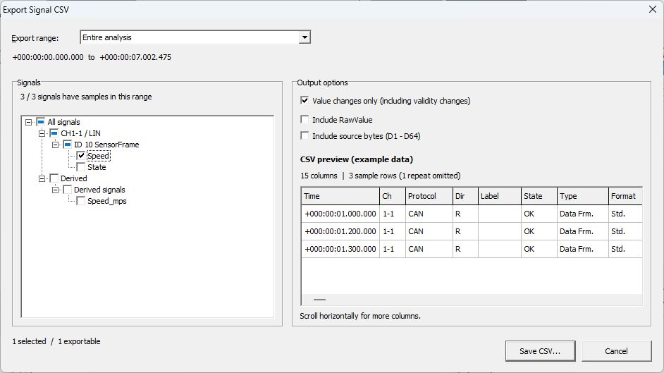
Figure 1. Normal export settings. The preview on the right uses fictional data.
| Item | Description |
|---|---|
| Entire analysis | Includes the entire analyzed range. |
| Current graph range | Includes the current graph display range. Check the selected Graph/Area first. |
| Selected trigger interval | Includes the selected trigger interval when available. |
| Tree under All signals | Selects signals to export from a hierarchy of channels, protocols, frames, and other items. [Outside this range] identifies signals with no samples in the selected range. [No analysis data] identifies signals with no samples in the entire analysis. |
| Value changes only (including validity changes) | On by default in Ver.4.10. Exports the first sample for each signal and samples where the value or valid/invalid state changed. Turn it off to export every sample. |
| Include RawValue | Adds a RawValue column. Derived signals have no Raw value as an original bus signal. |
| Include source bytes (D1 - D64) | Adds source frame data columns. |
Keep Speed checked and switch from “Entire analysis” (Figure 1) to “Current graph range” (Figure 2). Before opening the dialog, zoom Graph 1 / Area 1 to 0–1 s, before the first sample. The count of signals with samples changes from 3 / 3 to 0 / 3, while 1 selected stays unchanged and 1 exportable becomes 0 exportable. The tree shows [Outside this range], and “Save CSV...” is disabled.
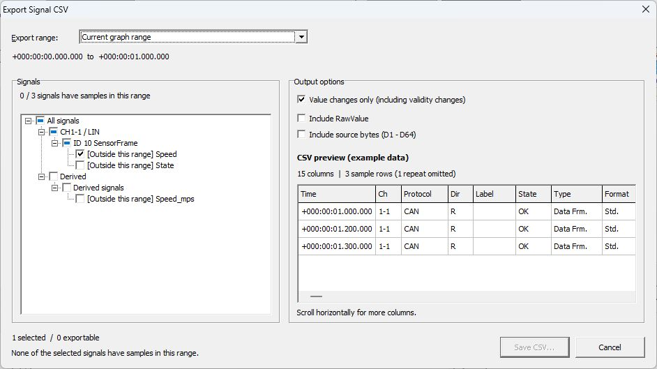
Figure 2. Changing the range changes sample availability and the exportable count.
“CSV preview (example data)” uses the fictional signal ExampleSpeed to show the output format. Toggle “Include RawValue” and “Include source bytes (D1 - D64),” then scroll horizontally to check the RawValue and D1–D64 columns. With “Value changes only (including validity changes)” on, the preview omits one of the four sample rows because its value and validity match the preceding row. Open the saved CSV to inspect the exported rows.
The CSV contains source frame information such as Time, Ch, Protocol, and ID, plus Signal, Value, Unit, SignalStatus, and DisplayText. For multiple signals, a separate row is output per signal for the same source frame. Check value validity together with SignalStatus.
Example: Comparing Exported Speed Values
Figure 3 shows an existing CSV export from a different Monitor buffer recording, opened in Excel. It uses Entire analysis with only Speed selected, Value changes only ON, and RawValue/source bytes OFF. Its recording times differ from Figures 1 and 2. To make checking easier, source-frame columns B–J are hidden and the Time column format is set to "+"0000000.000000. This adjusts the Excel display; it does not delete columns. The following table uses the same Time notation as Figure 3.
There are 6 samples, with Signal Speed, Unit km/h, and SignalStatus Valid throughout. Also check the correspondence between Value / Unit and DisplayText. The hidden source-frame information is Ch 1-1, Protocol LIN, Dir T, Type Response, ID 10 (hexadecimal 0x10), and DL 2.
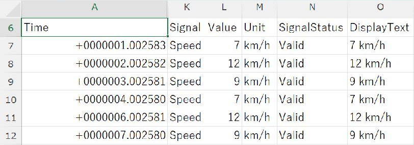
Figure 3. Formatting Time in Excel and checking Speed values, units, and Valid status.
| Time | Value (km/h) |
|---|---|
| +0000001.002583 | 7 |
| +0000002.002582 | 12 |
| +0000003.002581 | 9 |
| +0000004.002580 | 7 |
| +0000006.002581 | 12 |
| +0000007.002580 | 9 |
Since Value changes only is ON, duplicate samples in intervals that remain at 7 km/h are omitted. Row 8 in Figure 3 (+0000002.002582, 12 km/h) is the alert occurrence, row 9 at 9 km/h remains active, and row 10 (+0000004.002580, 7 km/h) is recovery. Check that timestamps and values match the occurrence/recovery history. You can also compare the waveform, Values, and Frame Log using Signal Analysis.
Checking the CSV Preview
Figures 4–6 are excerpts of the output options and preview. They use fictional ExampleSpeed data built into the dialog, rather than the analyzed LIN Speed values or a saved CSV. The example's Protocol is CAN; it does not change to match the analyzed log.
| Options | Preview columns / sample rows |
|---|---|
| RawValue OFF, source bytes OFF, Value changes only ON (Figure 1) | 15 columns / 3 rows (1 repeat omitted) |
| RawValue ON, source bytes OFF, Value changes only ON (Figure 4) | 16 columns / 3 rows |
| RawValue ON, source bytes ON, Value changes only ON (Figure 5) | 80 columns / 3 rows |
| RawValue ON, source bytes ON, Value changes only OFF (Figure 6) | 80 columns / 4 rows (includes 1 repeat) |
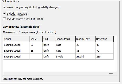
Figure 4. Adding RawValue. The invalid sample has an empty Value and RawValue 255.
Scroll horizontally to inspect source bytes. Figure 5 shows D1 as 28, 46, and FF (hexadecimal); the dialog adds D1–D64 columns.
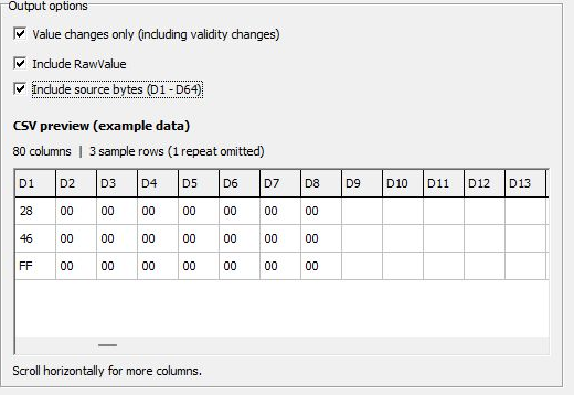
Figure 5. Adding source-byte columns to the fictional preview.
Turn Value changes only OFF to retain both consecutive samples at Value 20 / Valid, increasing the preview from 3 to 4 rows. Changes in validity are also retained when the option is ON. Check actual timestamps, values, and row counts in the saved CSV.
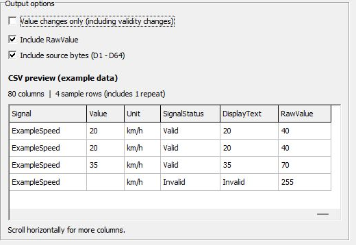
Figure 6. Keeping the repeated row in the fictional preview.
Example: Exporting Speed Within a Trigger Interval
This Ver.4.10 example uses a Monitor buffer recorded with ReTriggered, containing 14 frames and 3 trigger intervals. It is a separate recording from the 20–40 s Signal Trigger example in Monitor Trigger. Use the interval immediately before the last one.
- After stopping monitoring, analyze the Monitor buffer with Signal Set Default.
- In Graph 1 / Area 1, left-click a blank part of the target interval, such as around 4.5 s above the waveform. Clicking the waveform or legend selects a signal instead. The initial selection is the last completed interval; moving the time cursor alone does not confirm a change of interval.
- Open “Export CSV” and choose “Selected trigger interval.” Verify that the range is
+000:00:04.002.476to+000:00:05.002.478 (end excluded)(Figure 7). - Select only Speed under CH1-1 / LIN → ID 10 SensorFrame. There are 3 / 3 signals with samples; selected and exportable are both 1. Turn Value changes only OFF to retain every sample. Leave Include RawValue and Include source bytes OFF.
- Save as
ln1-trigger-previous-speed-samples.csvand inspect the actual CSV. The right-hand preview uses fictional data, so its 4 sample rows are not the exported row count.
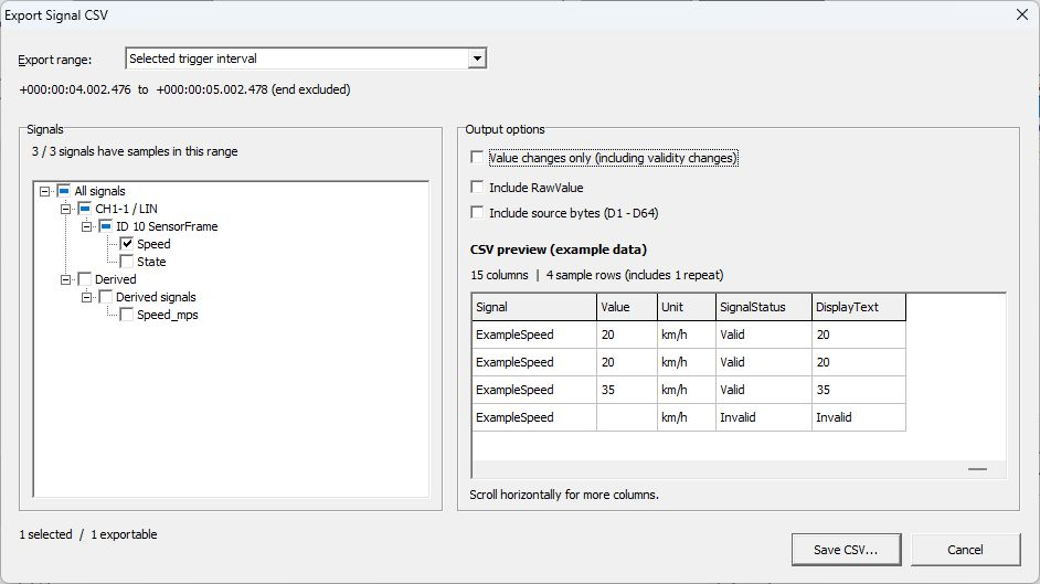
Figure 7. Export settings for the interval immediately before the last one.
The saved CSV contains 1 data row, excluding the metadata and column heading. Time is +000:00:04.002.476, Type is Response, Signal is Speed, Value is 7, Unit is km/h, SignalStatus is Valid, and DisplayText is 7 km/h. The sample at the start is included.
The source communication log for this interval, MPXLogData_1-1_0001.csv, contains 3 frames:
| Time | Type | D1 / D2 | Signal-value CSV for the selected interval |
|---|---|---|---|
| +000:00:04.002.476 | Response | 18 / 01 | Included: Speed 7 km/h |
| +000:00:05.000.762 | Header | — | No signal sample generated |
| +000:00:05.002.478 | Response | 22 / 01 | Excluded: at the end time, Speed 12 km/h |
The Header remains in Frame Log and the communication CSV but produces no signal-value row. The final Response remains in the communication CSV and is excluded from the selected-interval export because of end excluded.
For comparison, exporting the same Monitor buffer with Entire analysis, only Speed selected, Value changes only ON, and RawValue/source bytes OFF produces 7 data rows in ln1-entire-speed-samples.csv. The values are 7 → 12 → 9 → 7 → 12 → 9 → 7 km/h. All 7 rows are Response / Valid; each consecutive value differs, so Value changes only omits none of them.
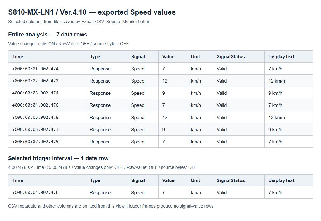
Figure 8. Selected columns from the actual exported CSV files, laid out for comparison. This is separate from the fictional preview in Figures 4–6.
Exporting Speed from a Saved LIN Communication Log
Open MPXLogData_1-1_0001.csv, the 3-frame communication log for the interval above, and compare it with the Monitor buffer export.
- Open the communication log with “Open Log.” Verify 3 frames, Signal Set Default, and 3 Matched signals in Log Analyze, then run Analyze. If changing the Set, follow Select the Signal Set for Analysis.
- In Frame Log, check the 3 frames in the table above: Response → Header → Response.
- Open Export CSV and choose Entire analysis. Select only Speed, turn Value changes only OFF, and leave RawValue/source bytes OFF. Save as
ln1-saved-log-speed-samples.csv.
The saved CSV contains 2 data rows:
| Time | Type | Signal | Value | Unit | SignalStatus |
|---|---|---|---|---|---|
| +000:00:04.002.476 | Response | Speed | 7 | km/h | Valid |
| +000:00:05.002.478 | Response | Speed | 12 | km/h | Valid |
Opening a communication CSV alone does not restore the Monitor buffer's trigger intervals, so Selected trigger interval is unavailable. Entire analysis includes the last Response in this saved log. The Header still produces no signal-value row. The 1-row and 2-row exports therefore have different ranges even though they use the same interval's communication data.
This CSV exports analyzed signal values for inspection in spreadsheet software and similar tools. Do not keep it instead of the original communication log or use it as a transmission log for Log Replay.
Saving Graphs as Images
- Select the target Graph and Area, then adjust the time range, axes, legend, and any required markers or annotations. This example displays CH1-1 Speed in Graph 1, Area 1 with Range 7.5 s. Also see Zooming In on Waveforms.
- Click “...” (More Graph commands) above the graph and select “Save Graph Area” (Figure 9).
- Select the destination, file name, and format, then save. Available formats are BMP, JPEG, and WMF. This example saves a BMP as
ln1-speed-high-graph-area-1.bmp.

Figure 9. Executing Save Graph Area for the selected Graph and Area.
- Open the saved image and check that the waveform, axis unit, legend, and time range are as intended. Figure 10 is the entire BMP saved by the application, losslessly converted to WebP for publication. It exports the selected Area's graph, not the Values, Frame Log, or Markers lists.
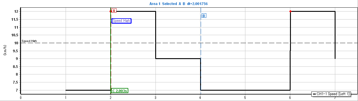
Figure 10. Checking the waveform and displayed content across the entire saved Graph Area.
In Figure 10, the vertical axis is km/h and the legend is CH1-1 Speed [Left 1]. The horizontal dashed line at 10 km/h is the Speed High upper limit; after the first red occurrence point, Speed changes 12→9→7 km/h. It remains active at 9 km/h around 3 seconds and recovers at 7 km/h around 4 seconds. The red point around 6 seconds is a separate occurrence. Compare exact occurrence/recovery times and values against Alerts and Frame Log or the exported CSV.
The green C 2.003 s, red A, blue B, and blue-bordered Speed High annotation are also retained in the image. The dt=2.001756 at the top is the A/B time difference, not the exact time from alert occurrence to recovery. Arrange the required displays before saving.
To keep an image for pasting from the clipboard, use “Copy Graph Area” in the same menu. The selected Area is copied as an image; check the target and content at the paste destination as well.
Include the log name, definition version, signal names, time range, and units with an image to help verify conditions later. An image alone cannot be used to reanalyze all original sample values.
Reusing Definitions
To reuse analysis definitions for monitoring, save MPXSIG on the analysis side and load it into the monitoring Catalog. This is separate from exporting communication logs or analyzed values.
- Stop monitoring and any running analysis, then open “Signal Catalog” within Signal Analysis. In the analysis Default [Current] in Figure 11, check the target definitions and Sets, then use “Save” to save as
ln1-speed-high-analysis.mpxsig. MPXSIG saves the Catalog and all Signal Sets.

Figure 11. Saving the analysis Catalog and Sets to MPXSIG.
- Open “Signal Catalog” from the monitoring Signal Window and first Save current settings under a different name. In this example, the 48 definitions and LIN Sensor [Current] before loading are saved to
ln1-monitor-catalog-before-reuse.mpxsig. - Use “Load” in the monitoring Catalog to select
ln1-speed-high-analysis.mpxsig. Check “Replace the Catalog and all Signal Sets?” in Figure 12; choose “Yes” to replace them or “No” to cancel.
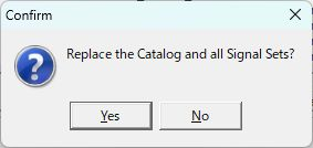
Figure 12. Confirming replacement of the monitoring Catalog and all Signal Sets.
- After loading, check Default [Current] and registered Speed, State, and Speed_mps in Figure 13. Check Speed's In Set enabled, Protocol LIN, ID (Hex) 10 (0x10), Message SensorFrame, and CH CH1-1. Also check waveform destination Graph On and Graph Area
G1 / A1.

Figure 13. Checking Current Set, channel assignments, and display destinations after loading.
- Select Speed and open “Edit” → “Alert” to check that conditions were also loaded. Figure 14 shows Speed High for Speed - Physical value, with Alert conditions 1 (ON: 1) and usage Monitor + Analysis. Range limits has Upper limit ON at 10 km/h, Lower limit OFF, Recovery margin 2, Notify Immediately, and Sound OFF. Compare against the same upper-limit monitoring condition.
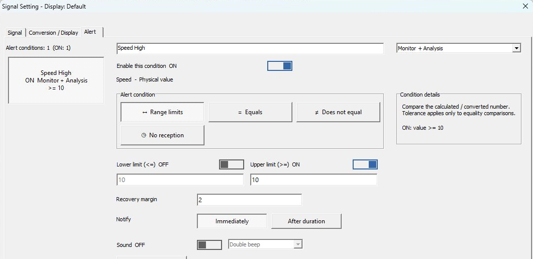
Figure 14. Checking alert conditions loaded on the monitoring side.
This does not simply add the selected Set. If any saved destination does not match the current device/channel configuration, channel assignments are cleared in all Sets. Check definitions and display settings and reassign channels for the signals you use. Closing with Close does not undo a confirmed load. For details, see Saving and Loading the Catalog.
For transmission use, see Integrating Signal Definitions with Transmission Settings. This does not automatically write analysis CSV values back to transmission settings.