Getting Started with Signal Analysis
Feature Overview
“Signal Analysis” in Analyze Window converts acquired communication logs using signal definitions, letting you compare values, waveforms, alert occurrences, and source frames. Use Signal Window for values during monitoring and Basic Analysis Operations for frame-level searching and combining.
Analysis requires a log and matching signal definitions. For signal terminology, see Signal Catalog Roles and Terminology.
See Changes in Ver.4.10 for the related screen and workflow updates.
Starting Analysis
1. Prepare a Log and Definitions
Stop monitoring and open “Signal Analysis” in Analyze Window. Analyzing saved logs does not require connecting a device or starting live monitoring.
- To investigate the most recent monitoring session, stop monitoring, open “Signal Analysis,” and check that “Source: Monitor buffer” is displayed.
- To investigate a saved log, use “Open Log” to open a MicroPeckerX communication log CSV. Spreadsheet CSV files and analysis CSV files cannot be used as source logs.

Figure 1. Checking the analysis Source and log summary.
Figure 1 uses the most recent monitoring log: Source is Monitor buffer, and the summary shows CH 1, records 14, and duration 7.002 s. trigger intervals is the number of trigger intervals in the log, which is 0 here. Check the number of detected alert conditions under Alerts in step 5.
If “Open Log” is canceled or loading fails, for example because a limit is exceeded, the previous log and analysis results are retained.
Starting a new monitoring session switches the analysis source back to the monitoring log and clears previous analysis results. Export any results you need before starting.
2. Select the Signal Set for Analysis
Prepare the analysis definitions
Saved logs use definitions from the analysis Catalog. To use the definitions from the time of capture, open “Signal Catalog” in Signal Analysis and use “Load” to load the MPXSIG saved with the log (for example, run.mpxsig for run.csv).
The first analysis after opening Monitor buffer imports the current shared Current Set. If differences from the definitions or channel assignments at monitoring start are reported, reselect definitions matching the log.
If a definition selection screen appears, choose one of the following.
| Operation | Definitions used |
|---|---|
| Use current Signal Set | Imports the shared Current Set with its saved channel assignments for analysis. Check correspondence with log channels. |
| Load Signal Set | Loads a saved MPXSIG for analysis. Select the version corresponding to the log. |
| Cancel | Cancels definition selection. |
Check the Set to use, In Set, and CH in the analysis Catalog. Match channels recorded in the log, not channel numbers of currently connected devices. Also compare Protocol, ID, Direction, and DL. If derived signals are included, check their input signals and formulas as well.

Figure 2. Checking signal membership, channels, and display destinations in the analysis Default Set.
The title in Figure 2 is Signal Catalog - Analysis (next analysis), with Default [Current] selected. Check Speed's In Set ON, Protocol LIN, ID (Hex) 10 (0x10), Message SensorFrame, and CH CH1-1. Speed, whose waveform is displayed, has Graph On and Graph Area G1 / A1. This example also adds State and derived signal Speed_mps to the Set.
Select the Set for the next analysis
When “Open Log” displays “Log Analyze,” check the Set name and “Matched signals.” To choose another Set or update the definitions, close “Log Analyze” with the × in the upper-right corner or press Esc. The log stays selected.
With monitoring and analysis stopped, prepare the definitions if needed and choose the Set from “Signal Set” at the top of Signal Analysis. Click “Analyze” in the same toolbar to run the analysis.
If you select another Set after analysis completes, “Signal Set” switches to the Set for the next run while the waveforms and Values still show the previous results. The selector is labeled “Signal Set (next analysis):”. “Export CSV” is disabled while reanalysis is pending. Click “Analyze” and confirm that the new results contain samples to export.
Example: Switching from Default to Speed Line
Figures 3–5 switch the analysis Set from Default to Speed Line with the saved communication log LN1_SpeedTrigger_1-1.csv open. This is a separate example from the Monitor buffer examples before and after it.
- Display the completed Default analysis and open
Signal Setat the top. Figure 3 offers Default and Speed Line. The displayed waveform uses Default's Stair mode.
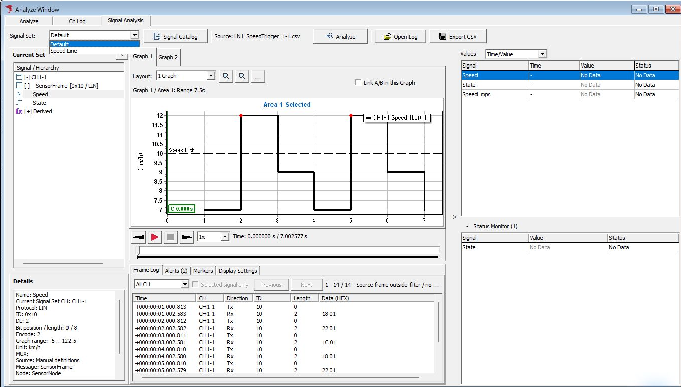
Figure 3. Choose the Set for the next analysis from the Signal Set selector.
- Select
Speed Line. In Figure 4, the next analysis Set changes to Speed Line, while the graph retains the previous Default Stair waveform.Export CSVis disabled. The selected Set name alone does not mean the displayed waveform has been updated.
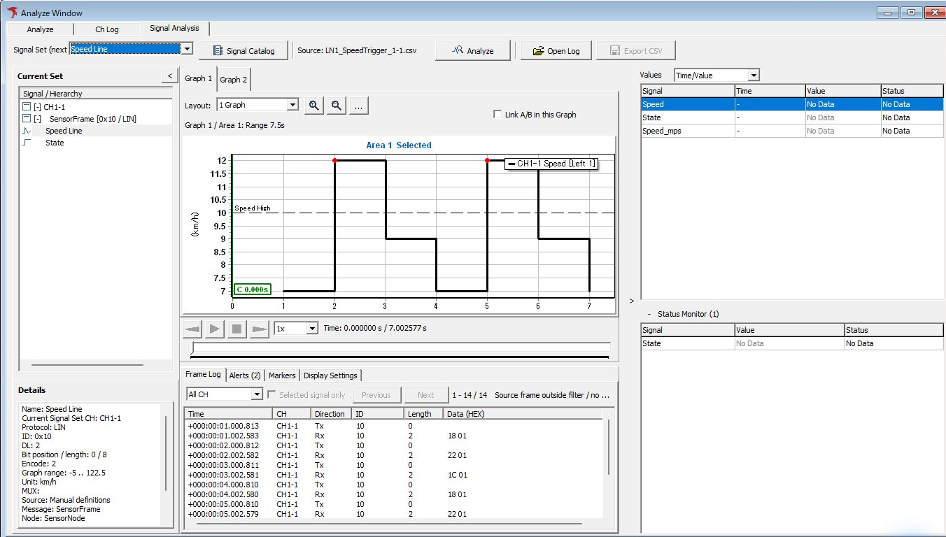
Figure 4. Reanalysis pending after switching Sets: previous results retained and CSV export disabled.
- Click
Analyze. On completion, the graph updates to Speed Line's Line mode, andExport CSVbecomes available if the results contain exportable samples (Figure 5). This capture clicksZoom Inthree times after reanalysis to set Range to 7.5 s. Also check the vertical-axis scale, signal names, Values, and Alerts against the new results and the selected Set's settings.
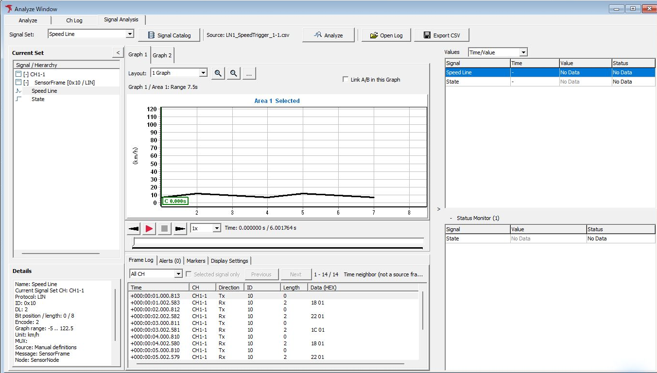
Figure 5. Check the Line display and enabled CSV export after reanalysis completes.
3. Run Analysis
If “Log Analyze” appears when opening a log, check the log, Signal Set, and Matched signals. If signals match, click “Analyze.” Also check the target channels and analysis time range.
If the target log is already selected, use “Analyze” at the top of Signal Analysis in Figure 6. This example has Monitor buffer selected as Source, so check the analysis Default Set, then run analysis with this button.

Figure 6. Analyzing the selected Monitor buffer using Analyze.
If Matched signals is 0, use “Open Signal Catalog” to review analysis definitions, Sets, and channel assignments. If the log itself has no frames, select another log.
4. Compare Values with Source Frames
After analysis, select the signal and timestamp to investigate, then compare Values, the graph, and data in Frame Log. Screen Layout and Waveform Inspection explains each region and marker operations.
Figure 7 double-clicks the Frame Log row at +0000004.002580. Check CH1-1, Direction Tx, ID 10 (hexadecimal 0x10), Length 2, and Data (HEX) “18 01”. Speed in Values on the right is 7 km/h at the same timestamp. First byte 0x18 is Raw value 24, matching 24 × 0.5 − 5 = 7 km/h. The green cursor C label 4.003 s rounds seconds to 3 decimal places.
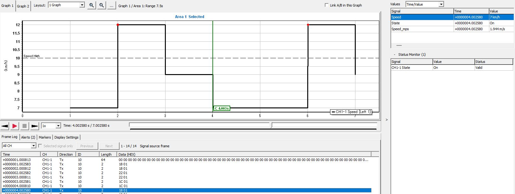
Figure 7. Checking the source frame, waveform, and Speed value at the same timestamp.
5. Rerun Analysis After Changing Conditions
| Entry point | Settings edited and where they apply |
|---|---|
| Signal Catalog on the main toolbar | Shared definitions used to prepare monitoring and transmission settings. Read-only while monitoring or analysis is running. |
| Signal Catalog within Signal Analysis | Analysis settings applied to the selected log. Cannot be operated while monitoring or analysis is running. Changes here are not written back to the monitoring Catalog or transmission data. After closing the analysis Catalog, check target signals and enabled states in Trigger Window before resuming monitoring. |
To change definitions used in existing analysis, confirm edits within Signal Analysis, close the Catalog, and run “Analyze” again. You can prepare changes in the analysis Catalog even while completed results are displayed. Old results remain while reanalysis is required, so complete analysis before comparing or exporting results using the changes. To retain old results, export CSV or images before changing conditions.
After reanalysis, check that Values and Alerts correspond to the changed conditions. Figure 8 shows Speed High results (upper limit 10 km/h, Recovery margin 2), with one Recovered and one Active event under Alerts (2). The top event occurred at 12 km/h and recovered at 7 km/h; the bottom event has not recovered by the end of the analysis range. Check target signals, condition names, occurrence/recovery times, and values, not just the count. For details, see Checking Alert Occurrences.

Figure 8. Example of checking conditions and detected results in Alerts after reanalysis.
To edit shared definitions, stop monitoring and wait for any running analysis to finish. You can edit while retaining analysis results. Changing shared definitions alone does not update retained analysis results or transmission data.
If Analysis Is Unavailable
| Situation | What to check |
|---|---|
| Analyze cannot be selected | Check that monitoring is stopped, a log is selected, definitions are ready, and no processing is in progress. |
| Matched signals is 0 | Check Set membership and the log's CH, Protocol, ID, Direction, and data length. |
| Signal values are missing or invalid | Check signal bit ranges, conversions, valid ranges, multiplexing conditions, and derived signal inputs. Do not interpret values before reception as zero. |
| Only waveforms are missing | Check Graph targets and Graph/Area assignments. Distinguish value analysis targets from waveform display targets. |
| Loading limit exceeded | Up to 5,000,000 frames across all channels can be analyzed. A CSV opened with “Open Log” must be no larger than 400 MB (400,000,000 bytes) and contain no more than 5,000,000 data rows across all channels, excluding the header. Split or reduce logs exceeding these limits and reopen them. |
Playback within the analysis screen moves the displayed time through analysis results. Its purpose differs from Log Replay, which actually transmits onto the bus. To retain results, see Recording and Exporting Results.